Parking in the typical urban environment is a huge annoyance and concern for most city dwellers, leading to a waste of time and fuel as well as an avoidable increase in pollution. Hence an interesting objective is to reduce the search time for parking in cities. This leads to the fundamental requirement of defining search time. Unlike its
Let us begin with a visual example from an experiment we ran to pin down search time definitions. Imagine several people sitting in a car and driving to a nice café in a crowded area of Berlin. Sadly, there are no free parking spots, so they have to circle around the block once to find a free spot and then walk back to the cafe. To track this process and provide ground truth readings, each person carried one or several smartphones (with GPS turned on) and used a customized app built on top of the predict.io SDK. This helped each user mark the time instant when s/he wished to start to search for parking and the time instant when the car was parked.
The SDK collects recordings from multiple smartphone sensors - GPS, accelerometer data, gyroscope, and others. The resulting annotated GPS traces for one particular trip is presented below:
It can be seen that the car enters the figure above from the top right corner, so we can see a colorful trace of differently sized triangles (the size represents the relative uncertainty in the GPS location reading, the orientation represents the GPS direction) approaching the marked "DESTINATION" in a counter-clockwise spiral. Even without the marker "manual parked" we can make out the location at which the car parked was by noting the point where the colorful traces becomes more wobbly and dense – indicative of people starting to walk.
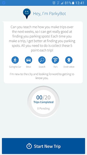
Fig. 1: ParkyBot Home Screen
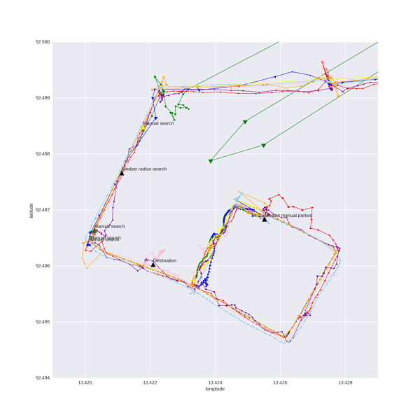 fig. 2: GPS Trace
It can be seen that the car enters the figure above from the top right corner, so we can see a colorful trace of differently sized triangles (the size represents the relative uncertainty in the GPS location reading, the orientation represents the GPS direction) approaching the marked "DESTINATION" in a counter-clockwise spiral. Even without the marker "manual parked" we can make out the location at which the car parked was by noting the point where the colorful traces becomes more wobbly and dense – indicative of people starting to walk.It can be seen that the car enters the figure above from the top right corner, so we can see a colorful trace of differently sized triangles (the size represents the relative uncertainty in the GPS location reading, the orientation represents the GPS direction) approaching the marked "DESTINATION" in a counter-clockwise spiral. Even without the marker "manual parked" we can make out the location at which the car parked was by noting the point where the colorful traces becomes more wobbly and dense – indicative of people starting to walk.
It can be seen that the car enters the figure above from the top right corner, so we can see a colorful trace of differently sized triangles (the size represents the relative uncertainty in the GPS location reading, the orientation represents the GPS direction) approaching the marked "DESTINATION" in a counter-clockwise spiral. Even without the marker "manual parked" we can make out the location at which the car parked was by noting the point where the colorful traces becomes more wobbly and dense – indicative of people starting to walk.
It can be seen that the car enrs the figure above from the top right corner, so we can see a colorful trace of differently sized triangles (the size represents the relative uncertainty in the GPS location reading, the orientation represents the GPS direction) approaching the marked "DESTINATION" in a counter-clockwise spiral. Even without the marker "manual parked" we can make out the location at which the car parked was by noting the point where the colorful traces becomes more wobbly and dense – indicative of people starting to walk.
It can be seen that the car enters the figure above from the top right corner, so we can see a colorful trace of differently sized triangles (the size represents the relative uncertainty in the GPS location reading, the orientation represents the GPS direction) approaching the marked "DESTINATION" in a counter-clockwise spiral. Even without the marker "manual parked" we can make out the location at which the car parked was by noting the point where the colorful traces becomes more wobbly and dense – indicative of people starting to walk.
Possible definitions of search time
There are several alternative definitions of search time of relevance to people
- the manual search time: this is the time difference between the point when a person "starts" to search, until the time the person reaches the destination. Although conceptually simple, it was observed (ref the 'Radius vs manual search time analysis' section below) that in
reality this definition left a lot open to interpretation and the consistency therein was not as high as anticipated. - the time interval between first entering within a circle radius of "R" from the destination point, to the time instant where parking is found (advantage: clearly defined and unambiguous).
- heuristic: the time interval between
a street X streets away from the destination point to the time at which you reach the destination.
In order to demonstrate a reduction in the search time, we evidently prefer a definition that has the following attributes
- clear to explain/ understand
- easy to compute
- as indicative of the perceptual feeling of search time as possible
- consistent: for a given definition of search time and under the same
real world conditions we would like the value of search time to be the same. Ofcourse as traffic conditions are not repeatable, in reality, this requirement means that the distribution of the search time for a sufficiently large number of samples taken over a sufficiently large duration of time does not change. This removes subjective definitions of metrics (such as a 1-10 rating based user feedback).
Further, if the manual search time can be replaced by an automated definition of search time (computable via sensor data), then this would yield significant savings in effort and time. As will be indicated below, this would also yield a greater certainty in these measurements owing to the inaccuracy in the manual readings recorded by users in tests. In addition, owing to safety reasons, in some experiments a user
Given our
- manual search starts are consistent across users
- manual and automatic search definitions are linearity related
Experiment and analysis
Setup of data acquisition
We identified locations in Berlin which, based on user experience, were difficult to find street parking in. Car-pools of users were deployed to find parking with a pre-specified set of locations (address/GPS locations). The users were given phone apps which would take user inputs on the following events
- start time of parking search
- time when the vehicle was parked
Both the driver as well as passengers indicated these events on their phones. Data was collected from over 50 phones over both Android and iOS devices on two different days. The visualization of one prototypical example trip is given above (Fig. 2).
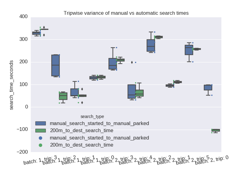
Fig. 3: Tripwise Search Times
Analysis of data collected
Radius vs manual search time analysis
We compared the automated definitions of search time against their manual counterparts. The data revealed that the radius based automated search times (green) show a lower variance than the manual search times (blue). This meets expectations, since the variance of the automated search time vary only by the devices' different GPS update frequencies, to calculate the time when a device first enters the given radius around the destination.
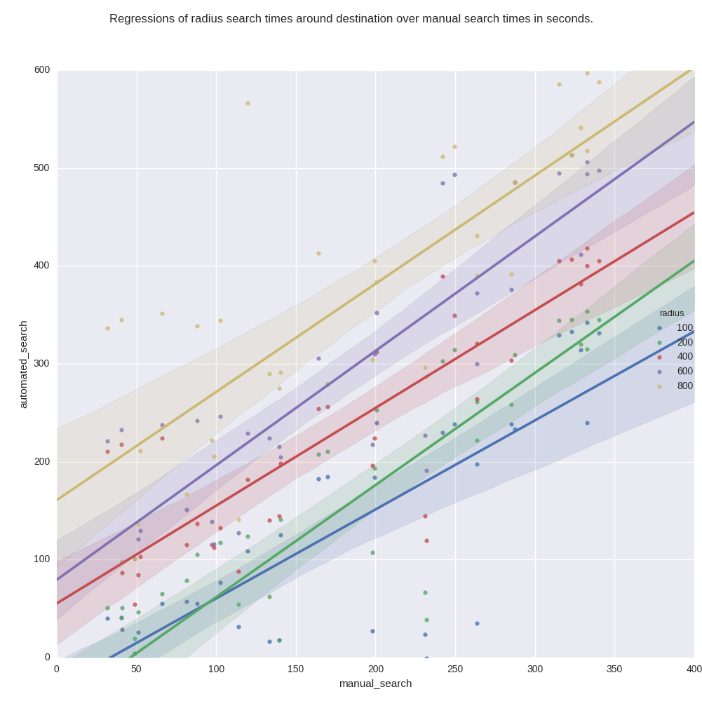
Fig. 4: Regressions destination
Linearity of search times
Given our desire to find a linear relationship between automated and manual search times, the following plots show this relationship for different radii used in the definition of the automatic search time. On the x-axis are manual search times, the y-axis shows radius search times. Different colors indicate the radii, that range from 100m to 800m.
As can be seen, higher radii lead to longer automated search times, as expected, since the car has to traverse a larger distance.
The following plots display the search times of two batches of data on two different days (with radii of 200m and 400m used in the automated search time definition). They reveal that the search times around the destination are not too stable across these batches.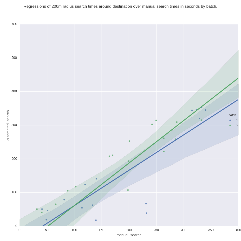
Fig. 5a: Regressions batch 200m
Fig. 5a: Regressions batch 200m
The above readings raise the following concerns:
- The offsets are not constant and might even change based on the day/location.
- A very small radius can lead to missing search
times, since a users phone might never have a GPS reading inside the circle (as happens when a radius of 100m is used in the search time definition). - In order to use the automated definition of search times to draw rigorous conclusions about the manual definitions, a large data size would be needed.
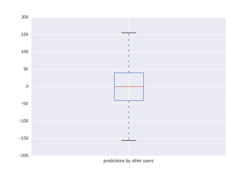
Fig. 6: User Agreement
Consistency of search times
In order to understand how well we are able to model manual search times, we ask the question "If we have Ann and Bob in the same car, how closely would Ann and Bob agree on when the start of
Author's notes: This might also have something to do with the fact that we discovered the surprising inability of one of our colleagues to parallel park in what we consider to be generously large spaces by the curb ;)
Lets now ask the following question "How well does our radius search start time model a single person's search start time?". To find an answer we observe the following box-plots of time differences between manual search starts and predicted radius search starts for different radii, again between 100 and 800m (Fig. 7a). Further, we are interested in the stability 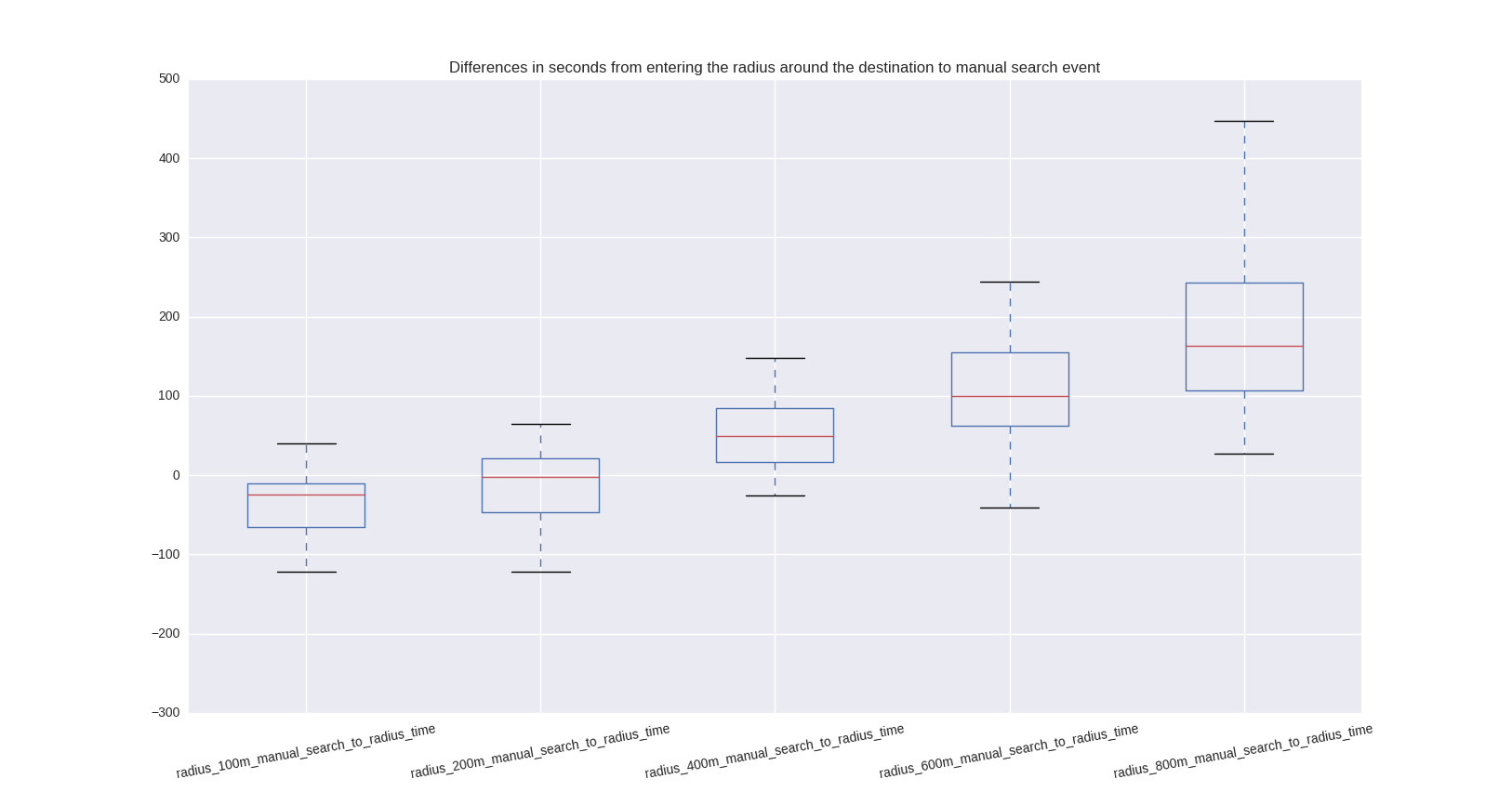
Fig. 7a: Time Differences
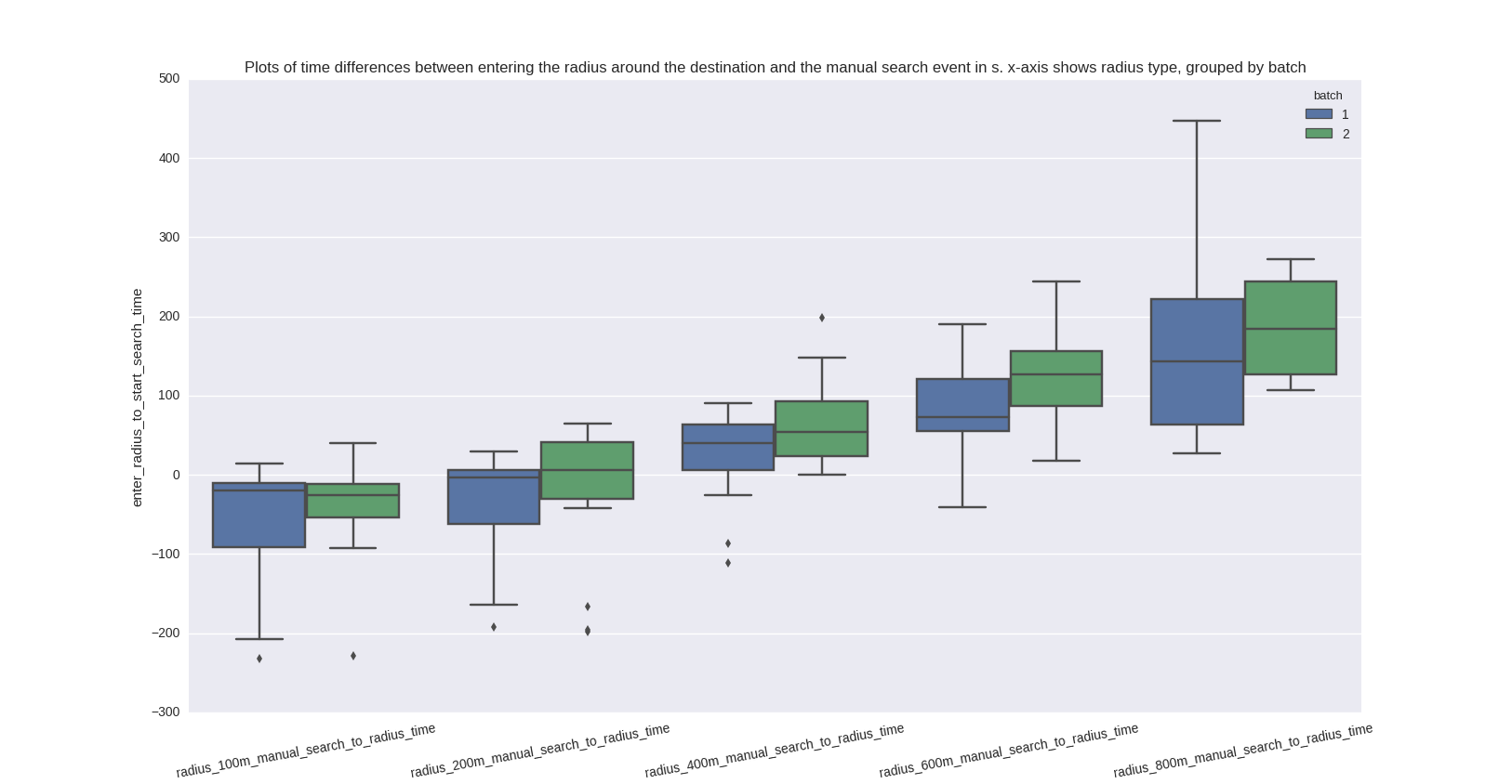
Fig. 7b: Time Differences Batch
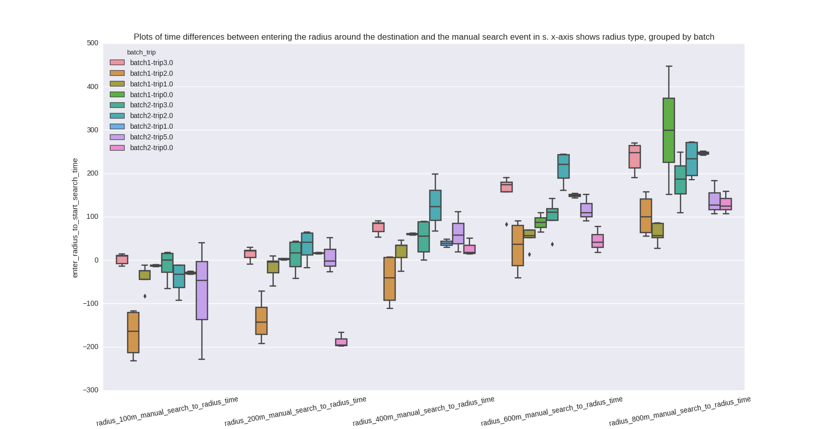
Fig. 7c: Time Differences Trip
Author's notes: These plots show that a radius of 200m when used in the automated definition, would model the search better than other radii. Surprisingly, it would even be more accurate than other people!
More precisely, the median distance between the 200m radius search time and the manual search times is zero, and 50% of the values lie outside the interval of -40s to +20s, which is slightly smaller than the 50% user agreement interval of -40s to +40s. But looking at the trip-wise distances we see that each trip behaves very differently. For example, batch1-trip2 and batch2-trip4 have an optimal radius at around 400-600m, whereas many other plots have an optimum at around 100-200m.
Insights
The above analysis yields the following insights.
- Manual search time variances are larger than anticipated - the perceived search times amongst users is significantly different even on the same trip! (See Fig. 6)
- Strikingly (as indicated in Fig. 7a for a radius of 200m) the median time difference of predicted start of search to the manual search time is zero. Also, the variance of the automated predictions against the user search times is slightly smaller than the user disagreement. This indicates that it is possible to approximate the manual search time using the automatic search time to within the experimental noise threshold. Hence it is feasible to estimate the manual search time with a linear function of the automatic search time. The suitable radius for this is 200-400m (Caveat: It is not certain that these findings will carry over to different cities.)
- As the destination is typically known, whereas the actual parked location might be uncertain when inferred, the automated search time defined using the destination is more stable.
- The automated search time (See Fig. 3) - is a more consistent and less subjective metric.
Conclusions
As we can see from this experiment, manual definitions of search time can be
Thanks for reading.
Arkadi Schelling, Machine Learning Expert @predict.io
Sridharan
